Literature review notes on automatic speech recognition

Deep Neural Network

Supervised Sequence Labelling with RNN (Graves)

• Ch. 2: Supervised Learning, Supervised Pattern Classification, Supervised Sequence Labelling
  • Pattern Classification (Recognition): Multilayer Perceptrons, Support Vector Machines.

Learning Phrase Representations using RNN Encoder-Decoder for Statistical Machine Translation (2014)

• Authors: Kyunghyun Cho, Bart van Merrienboer, Caglar Gulcehre, Dzmitry Bahdanau, Fethi Bougares, Holger Schwenk, Yoshua Bengio
• Amodei et al. cited this paper for GRU in Deep Speech 2 : End-to-End Speech Recognition in English and Mandarin.
• Encoder-Decoder model
• Objective function (maximize the conditional log-likelihood)

$$ \max_{\boldsymbol{\theta}} \frac{1}{N} \displaystyle\sum_{n=1}^{N} \log {p_{\boldsymbol{\theta}} (\boldsymbol{y}_n|\boldsymbol{x}_n)}, $$ where $\boldsymbol{\theta}$ is the set of the model parameters and each $(\boldsymbol{x}_n, \boldsymbol{y}_n)$ is an (input sequence, output sequence) pair from the training set.

• Gated Recurrent Units: reset gate and update gate.
• Some more explanation about GRU is available here.

Empirical Evaluation of Gated Recurrent Neural Networks on Sequence Modeling (2014)

• Authors: Junyoung Chung, Caglar Gulcehre, KyungHyun Cho, Yoshua Bengio
• Compare a long short-term memory unit, a gated recurrent unit, and a more traditional $\tanh$ unit
• A recurrent neural network (RNN) is an extension of a conventional feedforward neural network, which is able to handle a variable-length sequence input.
• Given a sequence $ \boldsymbol{x} = \left(\boldsymbol{x}_1; \boldsymbol{x}_2; · · · ; \boldsymbol{x}_T\right)$, the RNN updates its recurrent hidden state $\boldsymbol{h}_t$ by $$ \boldsymbol{h}_t = \left\{ \begin{matrix} 0, & t=0\\ \phi(\boldsymbol{h}_{t-1}, \boldsymbol{x}_t), & \text{otherwise} \end{matrix} \right. $$ Traditionally, the function $\phi$ is implemented as $$ \boldsymbol{h}_t = g\left( \boldsymbol{W}\boldsymbol{x}_t + \boldsymbol{U}\boldsymbol{h}_{t-1} \right), $$ where $g$ is a smooth, bounded function such as a logistic sigmoid function or a hyperbolic tangent function.
• RNNs can hardly capture long-term dependencies because the gradients tend to either vanish (most of the time) or explode (rarely, but with severe effects).
• LSTM and GRU are explained in detail in Chapter 3.

A time delay neural network architecture for efficient modeling of long temporal contexts (2015)

• Authors: Vijayaditya Peddinti, Daniel Povey, Sanjeev Khudanpur
• Two types of approaches to exploit long term temporal contexts are using feature representations or using acoustic models.
• Feature representations: 1. TRAPs 2. wavelet based multi-scale spectro-temporal representations 3. deep scattering spectra and 4. other modulation feature representations.
• original TDNN paper [Ref. 2].
• Sub-sampling: Asymmetric context windows of up to 16 frames in past and 9 frames in the future were explored in this paper. It was observed that further extension of context on either side was detrimental to word recognition accuracies, though the frame recognition accuracies improved (this phenomenon is widely known).

Token Passing Model

For me, I find it necessary to know how the Viterbi algorithm works in order to understand this token passing model. A good explanation in Chinese is available here.

Token Passing: a Simple Conceptual Model for Connected Speech Recognition Systems (1989)

• Authors: S.J. Young, N.H. Russell, J.H.S Thornton
• Introduction
  • One Pass and Level Building algorithms were essentially idential when syntax contraints were applied
• The central point of this paper is that token passing model leads to much simpler and more powerful generalization than lattice model. (p. 3)
• In order to understand the algorithm, readers need to keep in mind that tropical semiring is usually used in speech recognition. In tropical semiring, value $0$ denotes $\bar{1}$ and value $\infty$ denotes $\bar{0}$ [Reference].
• DTW is effectively a special case of HMM recognition.
• n-best token (p. 14)
• Conclusion: the advantage of Token Passing Model is that it has a clean interface and it is very straightforward.

Discriminative Training

Discriminative Training for Large Vocabulary Speech Recognition (2003)

• Author: Daniel Povey (Ph.D. thesis submitted to the University of Cambridge)
• A discriminative criterion called Minimum Phone Error is introduced in this thesis.
• 1986, Maximum Mutual Information (MMI, also known as Maximum Conditional Likelihood), 1993, 1997, Minimum Classification Error (MCE), Minimum Phone Error (MPE)
• Bayes’ rule (p.5, Fig. 2.2): prior probability, posterior probability
• Early HMMs use discrete output symbols, which were obtained by so-called “Vector Quantization”. At the moment essentially all work on speech recognition uses continuous vector-valued output symbols. (p. 8)
• History of speech recognition: 1968 (Dynamic Time Warping), 1975 (HMM, Dragon system), 1985 (GMM-HMM), 1985 (Replace whole-word models with phone models and context-dependent phone models), 1994 (Maximum A Posterior) & 1995, 1996 (Maximum Likelihood Linear Regression) for speaker adaption, 1994 (phone clustering), 1996, 1999 (Vocal Tract Length Normalization), 1998, 2000 (Linear Discriminant Analysis). Apart from the mainstream techniques, other directions of research have found use in small vocabulary systems.

Objective functions for training HMMs

• Standard objective function used in Maximum Likelihood Estimation

$$ \mathcal{F}_{ \text{MLE} }(\lambda) = \displaystyle\sum_{r=1}^{R} \log p_\lambda \left( \mathcal{O}_r | s_r \right), $$ where $s_r$ is the correct transcription of the r-th speech file $\mathcal{O}_r$. $\lambda$ denotes all the parameters of a set of HMMs.

• Maximum Mutual Information objective function

$$ \mathcal{F}_{ \text{MMI} }(\lambda) = \displaystyle\sum_{r=1}^{R} \log \frac{p_\lambda \left( \mathcal{O}_r | s_r \right)^\kappa P\left( s_r \right)^\kappa}{\sum_s p_\lambda \left( \mathcal{O}_r | s \right)^\kappa P\left( s \right)^\kappa}, $$ where $P(s)$ is the language probability for sentence $s$.

• Minimum Classification Error ojbective function

Why we need to use discriminative objective functions?

• The standard objective function has a strong assumption. Observation at time t depends on the corresponding hidden state only. This is not exactly true [Reference].

End-to-end speech recognition using lattice-free MMI (2018)

• Authors: Hossein Hadian, Hossein Sameti, Daniel Povey, Sanjeev Khudanpur
• Popular end-to-end approaches: (1) connectionist temporal classification (2) RNN-Transducers (3) attention-based methods
• Attention-based models have performed very well in a few tasks such as machine translation but, unless the training data is very large, they have not been as effective for speech recognition tasks [Ref. 6].

Weighted Finite State Transducer

Speech Recognition Algorithms Using Weighted Finite-State Transducers

Keyword Spotting

Small-footprint keyword spotting using deep neural networks (2014)

• Authors: Guoguo Chen, Carolina Parada, Georg Heigold
• Meaning of small footprint in terms of programming explained here.
• A commonly used technique for keyword spotting is the Keyword/Filler Hidden Markov Model.
• This paper proposes a Deep KWS system.
• The voice-activity detector is decscribed in Ref. 14: uses PLP features and GMM model.
• Deep KWS: 30 left-spliced frames, 10 right-spliced frames.
• HMM baseline: 10 left-spliced frames, 5 right-spliced frames.
• ReLU outperforms logistic activation function in their experiments.
• Compared the performance of four systems: HMM baseline (VS), HMM baseline (VS+KW), Deep (KW), and Deep (VS+KW).

Query-by-example keyword spotting using long short-term memory networks (2015)

• Authors: Guoguo Chen, Carolina Parada, Tara N. Sainath
• Goal: detect user-specified keywords
• Feature extraction: use 5 future frames and 10 past frames
• LSTM Feat Extractor outperforms Phone LSTM + DTW, and both of them outperforms Phone DNN + DTW
• Maybe LSTM is more robust than DNN in noisy environment?

Streaming small-footprint keyword spotting using sequence-to-sequence models (2017)

• Authors: Yanzhang He, Rohit Prabhavalkar, Kanishka Rao, Wei Li, Anton Bakhtin, Ian McGraw
• A streaming keyword spotting system using a recurrent neural network transducer (RNN-T) model was developed
• Baseline: CTC based keyword-filler model
• Best performance: false reject (FR) rate of 8.9% at 0.05 false alarms (FA) per hour (RNN-T phoneme with biasing)
• Attention mechanism was used to bias the RNN-T system towards a specific keyword of interest
• <eow> and <eokw> tokens can be helpful

Region Proposal Network Based Small-Footprint Keyword Spotting (2019)

• Authors: Jingyong Hou, Yangyang Shi, Mari Ostendorf, Mei-Yuh Hwang, Lei Xie
• Region Proposal Network (RPN) used in keyword spotting
• At a false alarm rate of 1/h, the authors achieved a false rejection of approximately 5% for ‘Nihao Wenwen’
• The dominant approach to small-footprint KWS was the keyword-filler Hidden Markov Model (HMM) [Ref. 4-8].
• HMM state posterior?
• Feedforward DNNs gave significant improvement over the HMM-DNN approach in low-footprint scenarios [Ref. 14-17].
• Source code: https://github.com/jingyonghou/RPN_KWS
• Feature extractor: GRU (after fbank)
• Baselines: (1) Deep KWS: spliced with 15 left frames and 5 right frames (2) RNN-attention (3) end-of-keyword labelling
• The finding that the DET curve for ‘Nihao Wenwen’ outperformed that for ‘Hi Xiaowen’ is likely because ‘Nihao Wenwen’ is longer (4 syllables instead of 3 syllables) and hence it is easier to distinguish ‘Nihao Wenwen’ from other non-keyword audio. 【这里提到了唤醒词的音节问题】

Multi-Task Learning for Voice Trigger Detection (2020)

• Authors: Siddharth Sigtia, Pascal Clark, Rob Haynes, Hywel Richards, John Bridle
• The baseline model architecture comprises an acoustic model (AM) with four bidirectional LSTM layers with 256 units each, followed by an output affine transformation + softmax layer.
• Results in two different test are shown in the figure below:
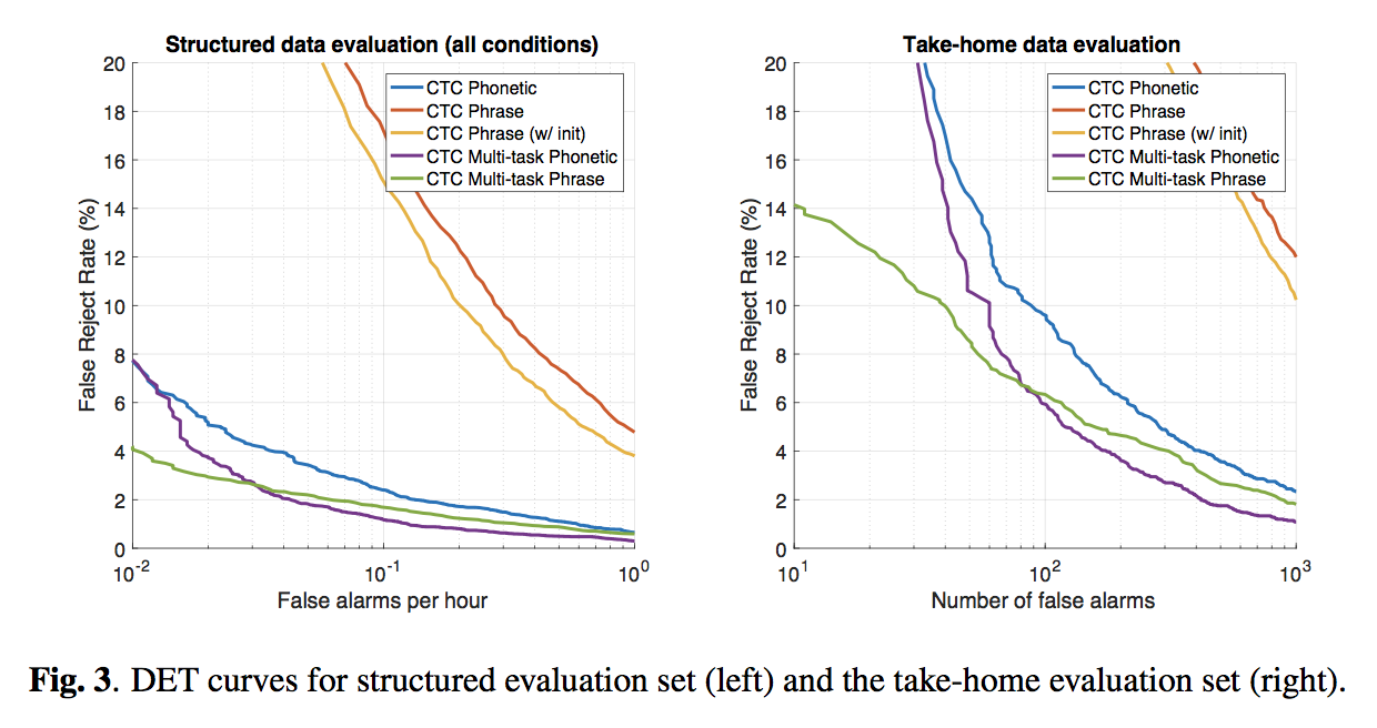
• It is important to collect dataset in real environments in order to measure unbiased false-reject and false-alarm rates for realistic scenarios similar to customer usage.

Far-field Speech Recognition

JHU ASpIRE system: Robust LVCSR with TDNNS, iVector adaptation and RNN-LMS (2015)

• Authors: Vijayaditya Peddinti, Guoguo Chen, Vimal Manohar, Tom Ko, Daniel Povey, Sanjeev Khudanpur
• This work compared the impact of input contexts, volume purterbation, iVector adaption, using pronunciation and silence probabilities in lexicon, and RNN-LMs on speech recognition.
• Reverberant speech is assumed to be composed of direct-path response, early reflections (viz. reflections within a delay of 50ms of the direct signal) and late reverberations (with reverberation time from 200 to 1000 ms in typical office environments).
• (Early reflections / Late reverberations) can be dealt with using DNN architectures which operate on comparatively (short / wide) temporal contexts.
• Sub-sampling is explained in Sec. 2.2.1.
• The prior term in the iVector extraction is quite important when applying these iVector based methods to data that is dissimilar to the training data.
• They found empirically that excluding the silence from the statistics for iVector estimation was very helpful.
• GMM-based VAD [Ref. 19].
• It worth mentioning that it is important to generate the N-best hypotheses with the optimal acoustic scale.

Reverberation robust acoustic modeling using i-vectors with time delay neural networks (2015)

• Authors: Vijayaditya Peddinti, Guoguo Chen, Daniel Povey, Sanjeev Khudanpur
• Similar to JHU ASpIRE paper.
• A potential drawback of the enhancement based approaches is the inevitability of estimation errors [Ref. 1].
• Their TDNN uses the p-norm non-linearity.
• semi-tied covariance (STC) transform [Ref. 30]